Hitesh Mittal / Kathryn Berkow / Johnson Zachariah
Introduction
Because the US equity market contains sixteen exchanges and thirty dark pools, choosing where to post limit orders is a complex problem for execution algorithms. Most broker execution algorithms leave this decision to a special class of algorithms called Smart Order Routers (SORs), and while they often contain dynamic logic for taking liquidity, logic for posting orders is often static and far less sophisticated. Many brokers provide their clients a choice of venues at which they can post, organized by themes such as “high-rebate venues”, “inverted venues”, “highest market share”, and “primary listing”, for example.
Static selections for routing limit orders can lead to significant performance degradation of execution algorithms. Orders posted by SORs can be “queue-jumped” by other market participants posting their orders in venues with higher preference for receiving marketable orders. Despite the Order Protection Rule of RegNMS, orders posted more passively can receive executions over orders priced more aggressively in certain cases, and limit orders that are pushed back in the queue face both lower fill rates and higher adverse selection. One of the most important factors in determining a venue choice for posting orders is “conditional fill rate”. Selecting a venue for a passive order is a complex problem because it depends on the specific exchanges competing at the NBBO at the time of order placement. The speed of a fill at NASDAQ depends not only on NASDAQ’s market share, but whether orders at the same price are also posted at IEX or EDGX, for example, or some other combination of three, eight, or fifteen other exchanges. And there are 65,535 possible combinations of exchanges that could be competing simultaneously at the NBBO, so a static or heuristic-based routing table cannot optimize limit order placement.
In this paper, we provide examples of “queue-jumping” within the existing US equity market structure and describe quantitative methods that help identify exchanges with the highest likelihood of filling limit orders given the set of exchanges at the NBBO. One method, ELO, is also used to rank chess players; players are assigned an ELO rating based on previous performance that can be used to compute the odds that one player wins over another—even if they have never played. We assign ELO ratings to each exchange and use them to quantify the odds that one exchange receives a trade over others based on their respective ratings. We also introduce a conditional fill rate matrix to determine optimal routing when posting limit orders. And finally, we share our observations of the characteristics that lead an exchange to become more competitive versus others based on the two methods.
The Problem
One of the motivating factors behind RegNMS was to encourage competition among exchanges, and it certainly seems to have achieved that as sixteen exchanges now compete for each order. This excessive fragmentation, however, makes it difficult to choose where to post a passive limit order without understanding how liquidity-taking orders on the opposite side may be routed by other market participants.
Price Priority is (Generally) Enforced
A critical feature of RegNMS—the Order Protection Rule—helps alleviate this concern at least partially. The Order Protection Rule was designed to break the monopoly of the largest exchanges by requiring brokers to take liquidity from an exchange that is providing it at the best available price—the National Best Bid (NBB) and National Best Offer (NBO) together form the National Best Bid and Offer (NBBO). All orders must be executed at the NBBO or better, and if a broker does not have the technology to connect to all exchanges they can route an order to any exchange—but that exchange must route the order to an exchange at the NBBO if it does not have that price available. Essentially, this means a limit order can be posted on any exchange, and as long as it is alone at the best price it will be first to trade against a marketable order on the opposite side1 (a market order to sell if the order is a limit order to buy, for example).
As a result of RegNMS, exchanges face fierce competition for market share and compete via access fees (i.e. offering a variety of fee structures for taking liquidity, ranging from rebates of 25 mills per share to fees of 30 mills per share), by creating new market structure innovations (e.g. IEX applies a brief pause to all orders and cancellations2), and by creating other incentives for large market makers and broker dealers. But if an order is alone at the best price, none of these features will detract from it being the first in the queue to trade against the next marketable order on the opposite side. There are some important caveats to this rule, however, described below.
No price protection on hidden orders
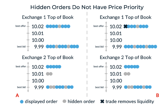
Hidden orders are not protected in the same way displayed orders are, described above. A hidden order is a non displayed order on an exchange that can receive price priority but is not published in the order book or included in the official BBO of an exchange (and thereby is also excluded from the NBBO). Consider for example, the NBB is 10.91 and the NBO is 10.99, and there are three exchanges competing at the NBB of 10.91—NYSE, NASDAQ, and IEX. Since the next marketable sell order will be routed to one of the exchanges at the NBB, a reasonable strategy might be to place a hidden order to buy at 10.92 at one of the exchanges at the NBB—NASDAQ, for example—in hopes that the order would intercept the next execution intended for the NBB. This hidden order would have price priority over other buy orders at NASDAQ at 10.91. But this would be a strategic risk; there is no guarantee that the marketable order would go to NASDAQ. If the marketable order goes to NYSE instead, then a trade would occur at NYSE at 10.91 and the hidden buy order at NASDAQ is left unexecuted. Had the hidden order been placed in the right venue (NYSE in this example), it would have traded because it would have price priority over other orders—unless there were other hidden orders at that price with time priority. As hidden orders account for an increasing portion of liquidity of US equity exchange volumes (recently averaging 16.7% for highly liquid stocks and 20.8% for illiquid stocks3 but varying widely across stocks and exchanges), the ability to predict which exchange will receive the next market order could be extremely beneficial for strategic hidden order placement.
Figure 1AB. Two hidden orders on Exchange 2offer improved pricing for the next arriving marketable order to buy (A). A market order to buy arrives at Exchange 1 (B), which has the NBBO, ignoring the hidden liquidity placed at a better price on Exchange 2.
No price protection on odd lots
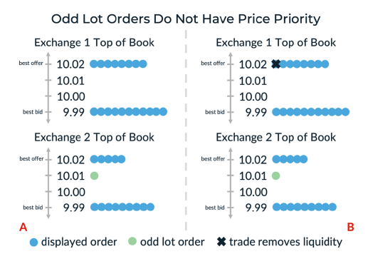
The Order Protection Rule of RegNMS applies only to round lot orders; there is no price protection for odd lot orders, even if they are displayed. Consider, for example, a trader buying Google stock, where NASDAQ is at the NBB at a price of 1450.50. The trader places an order of 50 shares to buy at NYSE at 1450.90, 40 cents higher than the NBB. A broker receiving a marketable order to sell may still send the order to NASDAQ, even though the order at NYSE is at the best available price, because the odd lot does not have the price protection round lots enjoy. NASDAQ is not required to route that order to NYSE to trade against the odd lot at the better price.
Figure 2AB. An odd lot order on Exchange 2offers improved pricing for the next arriving marketable order to buy (A). A market order to buy arrives at Exchange 1 (B), which has the NBBO, ignoring the hidden liquidity placed at a better price on Exchange 2.
Queue-jumping via a higher priority exchange
Even if the trader had improved the NBBO using a displayed order rather than a hidden order and it was a round lot order, there are some circumstances in which the order may not be the first in the queue. Each US equity exchange maintains price-time priority, meaning that orders placed first at a given price are traded first. While price priority is enforced across exchanges, time priority is not enforced across exchanges (for orders at a given price).
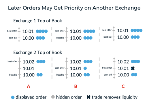
For example, assume that the NBB is 10.91 (and NBO 10.99), and NASDAQ is the only exchange at the bid of 10.91. A trader places an order to buy at NASDAQ at 10.92 to get price priority and that order becomes the first order at the new NBB. But another trader places an order for 10.92 at NSX after the order at NASDAQ. A marketable order to sell can now be executed at either NASDAQ or NSX—both at the NBB—even though the order at NASDAQ arrived first at the current best price. If a marketable order to sell arrives at NSX, the NASDAQ order will not receive a fill though it was first to place an order at that price, and the order at NSX receives the fill over the NASDAQ order without improving the price. This is referred to as “queue-jumping”. If the NBB moves up before the NASDAQ order at 10.92 is filled, that trader will likely need to reprice the order to match the higher bid or, worse, execute the order at the offer paying the full bid-offer spread.
Here again, reliably predicting which exchange will be most likely to receive an opposing marketable order would improve the likelihood and speed of execution of limit orders and avoid being jumped ahead of by other orders. In addition, those who can predict exchange priority could benefit from queue-jumping themselves, jumping ahead of orders with time priority at the same price. Reliable predictability of this depends on understanding how firms prioritize exchanges in their aggressive order placement via SORs.
Figure 3ABC. Exchange 1 is at the NBBO while Exchange 2 is at the NBB only (A). A limit order is posted at the NBO on Exchange 2 (B). A market order to buy trades against the new limit order at the NBO on Exchange 2 (C),jumping ahead of the orders placed before it on Exchange 1.
Queue-jumping via dark pools and single-dealer platforms
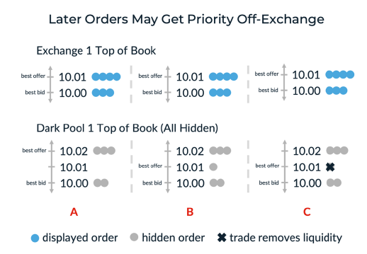
Within an exchange, hidden orders have lower priority than displayed orders; if a trader posts a hidden order at 10.91 and another trader later posts a displayed order at 10.91, the first order will be executed only after the displayed order is executed. This is intended to encourage market participants to contribute to the price discovery process. However, this rule does not apply across venues. Consider an order alone at the NBB of 10.91 at CHX when a broker receives a market order to sell. While the Order Protection Rule prevents the broker from executing the order at a price below the NBB, it does not mandate that the broker has to send the order to the exchange at the NBB. It is common for brokers to seek liquidity in dark pools and single-dealer markets first, and these venues may fill the broker order first—jumping the queue using a hidden order instead of a displayed order. Additionally, if the broker does not find liquidity in an off exchange venue but does not have connectivity to CHX, the order can be routed to an exchange not at the NBB. If the broker sends the order to NASDAQ, for example, NASDAQ has no obligation to send this order to CHX. Instead, NASDAQ can look for liquidity in dark pools or hidden liquidity within its own limit order book before routing the order to CHX, which is the only exchange at NBB. Thus, predicting which exchanges may be ranked lower in priority by broker SORs could help traders avoid the adverse outcome of slow (or no) execution even when priced most aggressively.
Figure 4ABC. Exchange 1 is at the NBBO while Dark Pool 1 is at the NBB only (A). A limit order is posted at the NBO in the dark pool (B). A market order to buy trades against the new limit order at the NBO in the dark pool (C),jumping ahead of the orders placed before it on Exchange 1.
The US equities market as a “Queue of Queues”
As a result of the complexities introduced above, it is helpful to consider the US equities market to be a “Queues of Queues” of bids and offers. Each exchange queue provides time priority to [displayed] orders priced at the same price. Price priority within an exchange is also maintained regardless of whether the order is hidden or displayed. However, select exchange queues may move faster than others if the marketplace favors that exchange over others. If we could predict which exchange queue is going to “win” the next marketable order, that information could be used in a number of ways:
• Jump the queue at other exchanges without improving the price
• Strategically place hidden orders above the NBB (or below the NBO) in prioritized exchanges • Place orders in multiple queues based not only on the queue lengths but also on the relative speed at which those queues are served (by marketable orders)
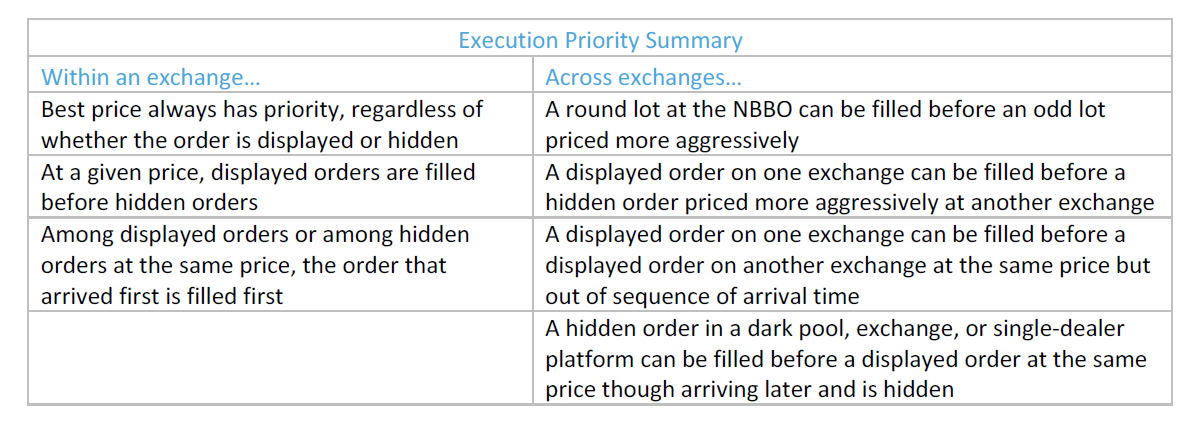
Regardless of preferred tactic, this information can help traders (SORs) make the most economical decisions in placing limit orders. For clarity, the execution priority of the “Queue of Queues” is summarized in Figure 5 below.
Figure 5. Execution priority rules governing the “Queue of Queues” within each exchange and across exchanges are summarized.
A Brief Introduction To Market Structure
The US equity market has 16 exchanges, twelve of which are owned by three “exchange families” NYSE, NASDAQ, and CBOE. There are four independent exchanges, namely IEX, MEMX, MIAX, and LTSE. Three of them—MEMX, MIAX and LTSE—only recently started trading and currently execute de minimis volumes. In addition to exchanges, there are thirty ATSs (dark pools) that represent approximately 10%4 of daily market volume. Similar to exchanges, most dark pools are limit order books with orders posted at various price levels either explicitly or referencing prices on exchanges (e.g. peg to bid); but all orders posted in a dark pool are hidden. Dark pools are operated by brokers, most of whom operate trading desks and execution algorithms and utilize their dark pools to cross clients’ orders. Finally, there are single-dealer platforms; these are not customer-to-customer platforms, rather they allow the operator (dealers or market-makers) to trade with clients directly (usually other broker dealers rather than buy-side institutions). These platforms represent the rest of the off-exchange volume (about 34% of daily volume).
Pricing
Exchanges offer three varieties of pricing:
• maker/taker—providing rebate to liquidity providing orders and charging a fee to liquidity taking orders
• inverted—reverse of maker/taker
• fee/fee—charging a fee to both sides of each execution
Both maker/taker and inverted exchanges aim to incentivize liquidity providers, but in different ways. Maker/taker exchanges incentivize liquidity providers by providing them a rebate, thus allowing them to earn returns in excess of the bid-offer spread. Though inverted exchanges charge liquidity providers a fee for posting liquidity, they help incentivize order flow by using the fee to fund a rebate to the liquidity taker. The idea here is that—all else equal—a liquidity taker would rather go to a venue that provides a rebate rather than charging a fee. In some ways, an inverted fee schedule is like a democratization of what is called “Payment for Order Flow” when market makers pay retail brokers to trade against their clients’ orders. Some market makers (“wholesalers”) provide liquidity to retail brokers and instead of charging a fee for liquidity (as in a maker/taker exchange) they provide a rebate to retail brokers to get access to that order flow. A summary of venues with corresponding market share and fee structure is shown in Figure 6.
Figure 6
Figure 6. This table illustrates the market share for venues in the US equities market, conglomerate affiliation, if any, and fee structure of each. Market share iscalculated from our sample data and may vary over time.
Pricing tiers
While exchanges are required to make their fee schedule public (unlike off-exchange venues), exchanges do discriminate based on complicated volume tiers. One broker may face an entirely different fee schedule than another for providing or taking liquidity because of the volume they trade. The pricing tiers are extremely complex to understand even though they are made available publicly5. Brokers may also hold interest in exchanges directly or indirectly6 and that may make the true economics of accessing these exchanges a bit different from merely the access fees.
Broker ATSs do not have a published fee schedule, rather they negotiate a price with each customer. Usually they follow a fee/fee model, similar to IEX. Brokers typically charge each other less than they charge asset managers, creating incentives for these brokers to route the flow to their dark pool before routing to the exchanges. Usually broker dark pools charge a fee between 5-10 mills per share, making them more affordable than maker-taker exchanges but more expensive than inverted exchanges. Alternatively, single-dealer platforms provide access to their liquidity for “free” (but earn spread) and sometimes even provide a rebate to brokers to access these platforms. They do so, in part, to create incentives for brokers to route orders to them before they route to exchanges—thus jumping the queue.
Why Typical Venue Selection Strategies are Suboptimal
With the considerations outlined above in mind, the question the rest of this paper will focus on is this: If there are multiple exchanges at the NBBO, which will be the first to receive a marketable order? If algorithm designers knew the answer to this question under a variety of circumstances, they could place limit orders on the appropriate exchange more often, thereby increasing the fill rate and fill speed of their limit orders and earning spread more reliably while trading. Naturally, there is no public information about how each broker, exchange, or other market participant routes their orders, whether by a static order or rule-based hierarchy. As a result, we aim to answer this question by analyzing TAQ data including every trade, all top-of-book quotes from each exchange, and each NBBO in the US equity market7.
Many market participants rely on market share as a method for deducing higher prioritization of a venue in SOR algorithms when posting non-marketable passive orders. While this would seem intuitive—that the higher the market share an exchange enjoys, the more likely other brokers’ routers are sending marketable orders to it—the data show that market share is a meaningful factor but is not sufficient for explaining the routing behavior of the marketplace alone. For Tape A securities, for example, NYSE has almost 16 times8 the market share of NSX and it is also the primary exchange—so we would expect NYSE to receive market orders more frequently than NSX. But a review of all such instances where NYSE and NSX were together at the NBB or NBO when a trade arrived9 reveals that NSX received the trade 63% of the time (and NYSE only 37% of the time).
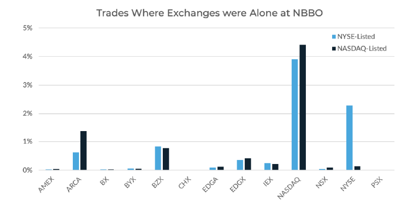
One reason market share alone is not sufficient for explaining routing preferences is because not all exchanges are competing at the NBBO at all times. At a given point in time there could be only one exchange at the NBBO, and if an order is routed to that exchange it is not a result of preference but because it is the only exchange at the best price. This happens only about 7% of the time overall and is shown in more detail in Figure 7. Similarly, there could be two exchanges at the NBBO where one may be preferred over the other, but both may be far less preferred than the other fourteen exchanges not at the NBBO.
Figure 7. This chart illustrates the percent of trades during which there was only one exchange at the NBBO, totaling just over 7%of the time for all Russell 3000 stocks. There is some variation when stocks are arranged by primary listing exchange, as shown here. Interestingly, there is very little variation across liquidity groups, with Russell 2000stocks having similar percentages to S&P 100stocks, though we might expect fewer exchanges to have the NBBO in less liquid names.
Another intuitive question would be whether access fees for incoming market orders would be enough to predict which exchange might receive the next order. Given that liquidity is available at the same price at multiple exchanges, it would be optimal for a broker to route market orders to the exchange that has the lowest access fee. But, like market share, we do not find that pricing alone is driving routing decisions, and there are other idiosyncratic factors likely involved. For example, IEX charges only 3 to 9 mills per share for market orders and NYSE charges up to 30 mills per share. It would be logical for a liquidity taker to take liquidity from IEX first and then NYSE if there are shares posted at the same price on both exchanges. But according to our analysis, when there was liquidity available at the same price at IEX and NYSE, a marketable order was routed to NYSE over IEX 63% of the time.
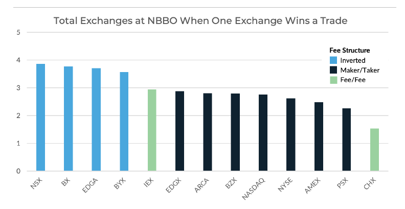
In fact, we observe from the data that each exchange faces a different amount of competition from other exchanges. Figure 8 captures the amount of competition each exchange faces on average for Russell 3000 constituent securities.
“Competition” here means the number of exchanges at the NBBO in total (including the winning exchange) when a trade is received by the winning exchange.
Figure 8. This chart illustrates the average number of exchanges competing (by having liquidity at the NBBO) whenever a particular exchange “wins” (executes) a trade. It also indicates the fee structure at each exchange. Inverted exchanges do appear to be preferred when competing, as market orders earn rebates on inverted exchanges.
The number of possible combinations of exchanges at the NBBO at any particular time makes it hard to analyze the routing preferences of the marketplace. There are a total of 120 combinations of any two of the market’s 16 exchanges being at the NBBO, 560 combinations of any three exchanges at the NBBO, and so on, yielding a total of 65,535 combinations possible. An algorithm, then, must be able to evaluate any combination of exchanges at the NBBO and decide where to place a limit order such that it will have the highest likelihood of being first to receive a trade.
Chess Players, Exchanges, and ELO
To simplify the problem and avoid evaluating all combinations, we use an approach inspired by a ranking system especially popular in the game of chess, called ELO. The ELO ranking was developed by chess player Emre Arpad Elo while he was president of the United States Chess Federation10. Each chess player is assigned an ELO score, and all players are initialized with a base of 1000. After a match, each player’s score is updated according to the formula shown in the Appendix. If a player’s pre-match ranking was lower and that player loses, their score remains largely unchanged, but a surprise victory improves the score more dramatically. An attractive feature of the ELO scoring method is that even if two opponents have never played directly, the odds for a winner can be estimated prior to their match. Consider the following example of a two-player game between Magnus Carlsen—Norwegian chess grandmaster with all-time high ELO rating of 288211—and an amateur, assigned a rating of 1000. Based on their scores, we can use the formulas detailed in the Appendix to predict the winner of a match between them, as shown below.
For a more exciting comparison, we can calculate the probability that Carlsen wins in a game versus Viswanathan Anand, currently rated 2753 (12th in the world).
There are many benefits of the ELO system. For example, though two opponents have never played, the odds of each player winning can be computed from a simple formula. Additionally, ELO can be computed in real time due to its iterative calculation, updating each time a game is played for an event-based status.
When it comes to exchanges, ELO can also be an interesting lens through which to view competition. Similar to the methodology described above for chess matches, we have analyzed exchange competition by assigning an ELO rating to each exchange and updating the rating of each following the arrival of each trade event within a trading day. Given the ELO scores of two exchanges, we can calculate the likelihood of one exchange winning the next marketable buy order over the other if both exchanges currently have available liquidity at the NBO, for example.
To rate exchanges, we initialized each exchange at the beginning of each trading day with an ELO score of 1200. When each trade arrived, we look at all exchanges currently competing at the NBBO. If the trade is at the NBO, we view all the exchanges at the NBO to be competing for that trade. Of course, only one exchange receives that trade and is declared the winner of the match. For instance, if NASDAQ, NYSE, and BATS all have the current NBO of $10.95 and a trade occurs at NASDAQ at $10.95, NASDAQ is assigned the winner of a match against NYSE and second match against BATS. The ELO scores of NASDAQ, NYSE, and BATS are updated accordingly. Note that if an exchange is alone at the NBBO and wins a trade, those “games” are not counted because there was no “competition”. Over the course of each trading day, the ELO scores of each exchange evolve into mature, well-defined scores12 ranking the exchanges. We performed this analysis both across stocks for all trades and within individual stocks.
An ELO Example
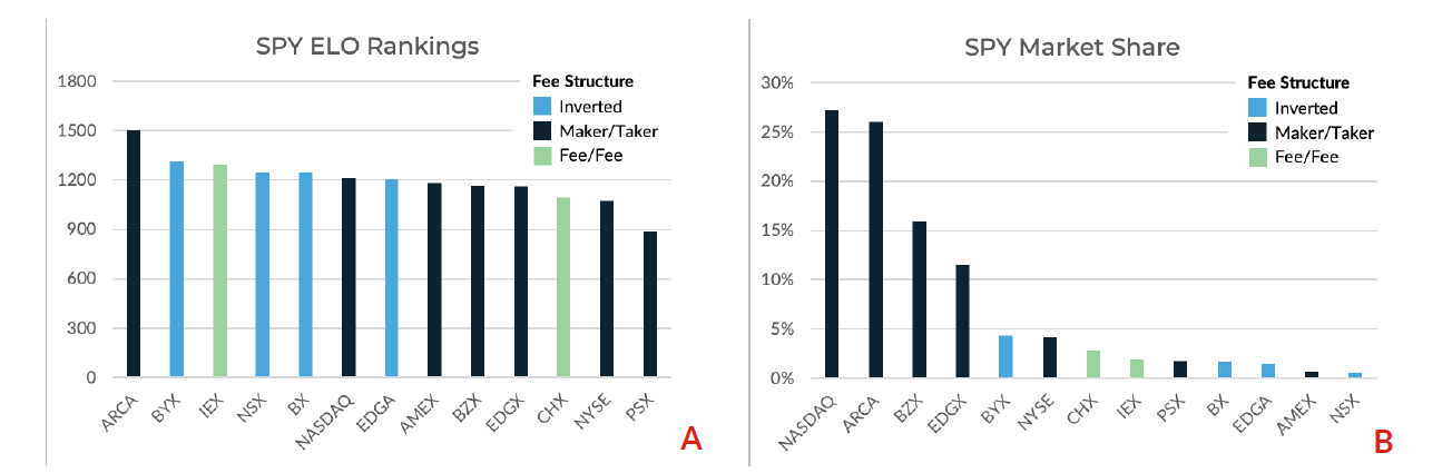
For a more specific example, the final ELO scores for S&P 500 Index ETF SPY are shown in Figure 9A and the off-exchange market share for varying exchanges for a single day in our sample data is shown in Figure 9B.
Figure 9AB. ELO rankings specific to SPY for each exchange (A) and market share specific to SPY for each exchange (B), including indication of whether each exchange is inverted, maker/taker, or fee/fee. Note that market share here excludes off-exchange volume.
As is illustrated in Figure 9A, inverted exchanges (in blue) tend to have higher ELO scores than other exchanges which shows that access fees are certainly an impactful factor in deciding the routing priority of the exchanges. However, that does not seem to be the only factor. For example, ARCA—the primary listing exchange for SPY—ranks highest overall though it has a very high access fee.
Market share also does not seem to explain ELO scores alone. The market share for SPY is shown in Figure 9B which indicates that NASDAQ has a higher market share than ARCA (though their access fees are similar). And yet, our data shows that when the two are competing at the NBBO for a marketable order, ARCA’s odds of winning a trade over NASDAQ is almost 85% versus NASDAQ’s 15%. In fact, for this particular example, the correlation of the ELO score with market share across exchanges is only about 41%.
Using ELO for Routing Decisions
From this example of just a single security, it is clear that one of the benefits of using the ELO ranking system to evaluate exchanges is its incorporation of the many important market dynamics—access fees, primary listing, market share, and more—that go into participants’ routing decisions for a quantitative, empirical, but also simple ranking to guide our posting strategy for optimal fill rate and speed.
Queue-jumping via hidden orders
Converting the ELO scores to probabilities indicating the likelihood of “winning” a trade is a simple calculation, as illustrated for the chess players above. Consider a scenario where ARCA and EDGX are the only two exchanges at the NBB and a trader wants to place a hidden buy order above the NBB to jump the queue. The likelihood that the next marketable sell order arrives at ARCA based on these ELO scores (ARCA’s score of 1504 and EDGX’s score of 1160) is 88% vs. EDGX’s 12%13. In this case, the trader has a higher likelihood of a speedier fill posting the hidden limit order at ARCA, but may choose to post at both exchanges if the order is large enough. Conversely, if the trader chooses to place the hidden order at EDGX, there is an 88% chance that an order priced more passively will receive a fill first at ARCA.
Queue-jumping via displayed orders
If placing a displayed buy order at the NBB, we can extend this method to incorporate ELO (fill speed), queue size, and rebate on each exchange to determine the optimal combination of venues. A simple algorithm like the one below can be highly effective in maximizing fill rate and minimizing access fees:
• Identify all exchanges at the NBB
• Identify the exchange with the highest ELO—call it the “likely winner”
• Identify those exchanges NOT at the NBB (thus having a queue of length zero) but with higher ELO scores than the “likely winner”
• Among these exchanges, identify the exchange with the lowest access fee to post an order
Similarly, tactics can be devised for optimal posting on multiple exchanges based on current queue sizes and ELO scores of each exchange.
Limitations of ELO
The iterative nature of ELO makes it a powerful method for estimating the likely fill speed of exchanges in real time when there is any arbitrary combination of exchanges at the NBBO, but it does suffer limitations in making such considerations across a group of stocks. For example, we wanted to study the difference in fill speed among exchanges based on primary listing exchange and liquidity. But ELO scores for each stock cannot simply be combined to derive such statistics because the range of ELO scores for each stock across exchanges can vary drastically. For one stock ELO could range from 800-1300, and 800-1600 for another. We normalized the ELO ratings for each stock to create a standardized ELO score across a group of stocks, but one cannot derive the specific odds of winning between two exchanges with normalized ELO scores using the formulas in the Appendix once the fundamental structure of the score has been changed. Normalized ELO scores can only be used for strictly ranking the exchanges and identifying “most likely”, “least likely”, or “more likely”, for example. While the relative rankings are somewhat informative, it is more useful to have the actual odds of an exchange winning a trade to inform passive order routing decisions.
An Alternative with Benefits: The WinMatrix Method
To address concerns about using the ELO scoring method across stocks, we have also developed a comprehensive approach that is measured on a fixed range of probability from 0 to 1 and comparable across stocks. We call it the “WinMatrix” method.
For every pairwise combination of exchanges and for every Russell 3000 constituent stock, we observe the number of times a trade occurred while the exchanges were both competing at the NBB (if the trade occurred at the NBB) or the NBO (if the trade occurred at the NBO)—the total “games played” by these two exchanges. If for example, if NASDAQ, NYSE, and EDGA are at the NBB and a trade occurs at the NBB on EDGA, this is counted as a game played between EDGA
and NASDAQ and a game played between EDGA and NYSE, where EDGA wins in both cases (very similar to the ELO method). No game is counted between NASDAQ and NYSE because neither is a winner. Following this methodology for each stock and counting such “games” for every trade in our sample yielded over 159 million observations (20 billion shares and more than $1.1 trillion). As a result, for every stock and every pairwise combination of exchanges, we recorded the total number of times the exchanges were together at the NBBO (“playing” or “competing”) and the number of times each exchange won the trade while they were together at the NBBO (“winning”). The ratio of the two yields the likelihood of each exchange being the winner of a single game played by the pair.
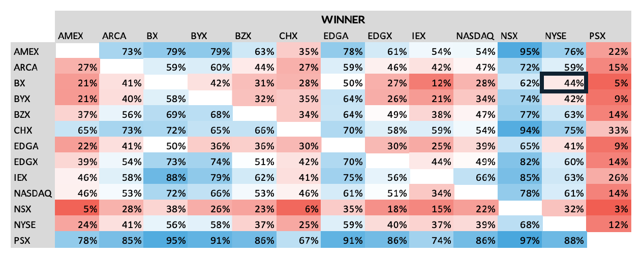
The strength of the WinMatrix method over ELO is that we can examine behavior by category of stocks, by simply aggregating the performance across stocks within a category for each pairwise combination of exchanges. The result of such aggregation is shown in Figure 9 below, which highlights the WinMatrix for liquid NYSE-listed stocks—those included in the S&P 100 Index. Each number in the matrix represents the percentage of games the exchange indicated by the column label is likely to win over its competitor (indicated by the row label).
For example, for the case outlined in the navy blue box in Figure 10, 44% is the likelihood that when NYSE and inverted exchange BX are both at the NBO or NBB and a marketable trade (to buy or to sell, respectively) arrives at one of the two, it arrives at NYSE. The matrix has a symmetric property; the entry at the location with NYSE as the row header and BX as the column header indicates that BX will win this face-off 56% of the time (100%-44%).
Figure 10. The WinMatrix for NYSE-listed S&P 100 constituent stocks. Each number in the matrix represents the percent of games the exchange indicated by the column label is likely to win over its competitor indicated by the row label. For example, for the case outlined in the navy blue box, 44% is the likelihood that when NYSE and inverted exchange BX are both at the NBO or NBB and a marketable trade (to buy or to sell, respectively) arrives at one of the two, it arrives at NYSE.
The WinMatrix is intimidating to observe with the human eye, but trading software can easily process this information and use it to facilitate the optimization of routing decisions. To make it easier to visualize these results, however, we can do a number of things.
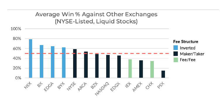
First, the WinMatrix can be collapsed to a strict ranking—more like the ELO scores—by taking the average win percent within each column as illustrated in Figure 11. The value of 79% indicated for NSX means that NSX wins a trade over other exchanges an average of 79% of the time when both are competing. What is most interesting in these results is that inverted exchanges have the highest average win frequencies, and that they are in order of the rebate each provides—NSX offering the largest rebate at 30 mills per share, and BYX offering the smallest rebate at 5 mills per share.
Figure 11. WinMatrix results for all exchanges for NYSE-listed, S&P 100 constituent stocks. The value of 79% indicated for NSX means that NSX wins a trade over other exchanges an average of79% of the time when both are competing(present at the NBO or NBB). The orange line is a reference indicating 50%. Note that inverted exchanges have the highest win frequencies, and are arranged in order of their take rebates, with NSX rebating 30 mills per share and BYX 5 mills per share.
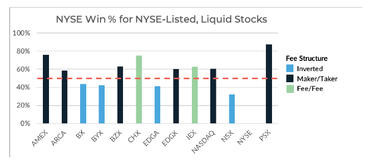
Another option that better preserves the benefit of the baked-in granularity in these measurements is to consider one exchange at a time, as we have represented for just NYSE’s performance for NYSE-listed, liquid stocks in Figure 12 below. The value of 76% for AMEX indicates that when AMEX and NYSE are competing (both present at the NBO or NBB), NYSE wins the trade 76% of the time. The solid orange line in Figure 12 is a reference line for 50% likelihood of winning when competing with NYSE. As indicated by the blue bars in Figure 12, inverted exchanges outperform NYSE for NYSE-listed stocks, each falling below the reference line. NSX is clearly the best location to post a limit order for the highest likelihood of earliest fill. When NYSE competes with NSX it has only a 32% chance of winning the trade. However, NYSE does perform better than all non-inverted exchanges, including those with substantially lower access fees.
Figure 12. WinMatrix results including only NYSE performance versus all other exchanges for NYSE listed, S&P 100 constituent stocks. The value of 76%indicated for AMEX means that NYSE wins a trade over AMEX 76% of the time when both are competing (present at the NBO or NBB). The orange line is a reference indicating 50%. Note that all inverted exchanges fall below the reference line, meaning that when competing with an inverted exchange, NYSE wins the trade less than 50% of the time for these stocks.
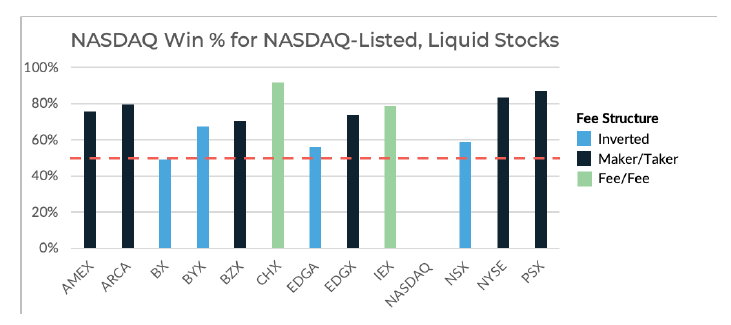
Similarly, the results for NASDAQ’s performance against competing exchanges for trades in NASDAQ-listed S&P 100 constituent stocks are illustrated in Figure 13. But here, we do not see that NASDAQ underperforms all inverted exchanges in its own names as NYSE does, rather it outperforms all but one—BX.
Figure 13. WinMatrix results including only NASDAQ performance versus all other exchanges for NASDAQ-listed, S&P 100 constituent stocks. The value of 76% indicated for AMEX means that NASDAQ wins a trade over AMEX 76% of the time when both are competing (present at the NBO or NBB). The orange line is a reference indicating 50%.Note only one exchanges falls below the reference line, meaning that when competing with inverted exchange BX, NASDAQ wins the trade less than 50%of the time for these stocks.
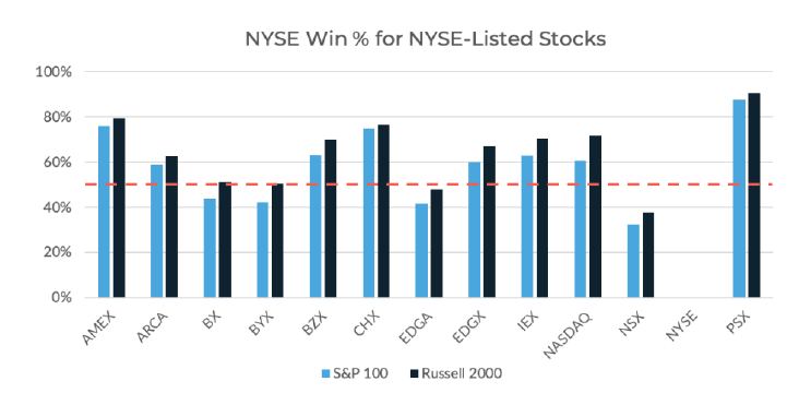
While one might expect to see a difference between liquid and illiquid stocks in exchange preference, Figure 14 shows NYSE’s performance for NYSE-listed names comparing S&P 100 stocks to Russell 2000 stocks. Clearly, no such different exists. The behavior variations across listing exchanges are the most dramatic we have detected in our study, which we believe is a direct result of legacy routing behaviors. We believe the stability of the WinMatrix across a variety of conditions underscores its value. Generally speaking, it doesn’t matter which group of stocks we’re looking at; the distribution remains the same.
Figure 14. WinMatrix results including only NYSE performance versus all other exchanges, comparing S&P 100 to Russell 2000 constituent stocks. The percentages indicated for AMEX indicate the frequency NYSE wins a trade over AMEX when both are competing (present at the NBO or NBB). The orange line is a reference indicating 50%. The results do not change much across liquidity groups.
Conclusion
Here, we have presented the challenges and opportunities that the US equity market’s fragmentation creates in optimizing venue selection for limit orders. Non-fragmented markets generally follow a price-time-display priority structure, where better-priced orders get executed first, displayed orders posted at the same price fill in the order they arrive, and hidden orders fill after displayed orders. But in our fragmented equities market, limit orders placed by execution algorithms can be jumped ahead of by other limit orders priced at the same or more aggressive pricing using a variety of techniques. If not routed optimally, orders can lose the opportunity to be filled when prices are preparing to move in their favor, resulting in both adverse selection and higher spread costs.
To answer the question of how best to route limit orders, we have presented two frameworks for estimating the odds that one exchange will win a trade over others, given the set of exchanges at the NBBO. The first framework is based on the ELO ranking system designed for rating chess players and frequently used in a variety of contexts, assigning an evolving and comparable rating to each exchange. Given the ELO scores of two exchanges, the odds of one exchange winning the trade over other exchange can be determined using a simple calculation. ELO is a useful framework because of its iterative approach and ease of calculations in real time, but it suffers a lack of generalizability over a group of stocks. The second framework—our WinMatrix method—requires more computation and more data storage but is far more robust for empirical analysis of exchange competition across stocks.
We know there are many factors brokers are likely using to determine their routing strategy for marketable orders— including market share, access fees, volume tiers, connectivity, skill of brokers’ routing strategies, and brokers’ own incentives to name a few. To fill passive orders quickly, one needs to align their limit order placement strategy with the marketable order routing strategy of other broker-dealers. Both the ELO and WinMatrix methodologies provide a useful way to identify the odds of that one exchange wins the next trade over the other exchange, while also illustrating that simply using market share and/or access fees alone cannot accurately predict routing behavior.
With the goal of navigating such complexity, we have presented various tactics that can be deployed to avoid losing priority to other market participants’ limit orders (or to secure priority over others’ orders). Our predictive frameworks and tactical strategies may also be useful for regulators in determining the role fragmentation plays in price discovery and studying incentives for brokers routing market orders to exchanges. In addition, they may be useful to exchanges looking to determine and improve the competitiveness of their limit order books versus the wide competitive landscape of the US equity market structure.
Appendix
Additional information about the ELO ranking system
The ELO ranking was developed by chess player Emre Arpad Elo while he was president of the United States Chess Federation14. The development of his method centered on the idea that players’ performance varied from game to game and day to day, but that in general, a very skilled player should have a strong likelihood of beating a less skilled player in a one-on-one match.
Each player is initialized with a fixed average score, say 1000. After each match, each players’ scores are updated according to the formula shown below. If a player plays as expected, their score will be relatively unchanged, but a surprise victory will affect scores more dramatically.
Probability Player 1 wins = 1 / (1 + 10^((Player 2 current score – Player 1 current score)/400)) Probability Player 2 wins = 1 / (1 + 10^((Player 1 current score – Player 2 current score)/400))
While two opponents may have never played before, there can be a clear expectation for a winner among them. This is a clear benefit to the ELO rating system; it can be used to rank players who have not faced off personally or both played another counterparty—a common ranking strategy in other sports.
The value of 400 is a constant in the ELO formula, specifying a fixed relationship between scores and probability15 and allowing for appropriate granularity of scores.
If Player 1 wins, the ELO ratings would update after the match as follows:
Player 1’s new score = Player 1’s pre-match score + 10*(1 – Player 1 win probability)
Player 2’s new score = Player 2’s pre-match score + 10*(0 – Player 2 win probability)
If Player 2 wins, the ELO ratings would update after the match as follows:
Player 1’s new score = Player 1’s pre-match score + 10*(0 – Player 1 win probability)
Player 2’s new score = Player 2’s pre-match score + 10*(1 – Player 2 win probability)
How much the score reacts to a win or loss after a match depends on the selection of the value of the “10” in the formulas above. This value can be selected by the user of the ranking system or even within a ranking system for scoring newer or more experienced players. Lower values of this constant will allow for slower changes in scores (accounting for past performance over a longer horizon) while higher values (e.g. 30) will allow for faster domination of the sport by a new player. For our analysis, we have fixed this constant, k, at 10.
Because of the initialization at a score of 1200, the center of the distribution, some exchanges will not play enough games (were not present at the NBBO frequently enough) in all symbols to develop a truly representative score. Our methodology eliminates an exchange for a particular symbol if it received fewer than 100 trades per day. If we did not remove such anomalies, these exchanges would have a relatively good ELO score of 1200 but would not have earned it.
End Notes
1 To enjoy order protection, an order must be a round lot. Round lots are sized at 100 shares for most stocks.
2 IEX has also recently released a new order type called D-Limit which automatically reprices to avoid trading just before a price change that would adversely select the order.
3 These values represent the total percentage of hidden volume each day for each security across all exchanges, averaged across days and then across symbols in the [most recent available] June 2020 data provided by SEC.gov.
4 This is calculated from the sample data used for this analysis but varies from day to day depending on market participant behaviors.
5 See for example the pricing schedule for NASDAQ and for NYSE.
6 MEMX, for example, was owned entirely by brokers, banks, and other market participants when it launched in early 2019.
7 The sample data for this analysis includes all top of book quote and all trade data for each exchange for five complete trading days in August 2020.
8 For Tape A stocks within the Russell 3000, NYSE’s market share averages 20.5% of daily volume and NSX’s is 1.3% in our sample. 9 This analysis includes all instances where both NYSE and NSX held visible available liquidity at the NBB when a marketable order to sell arrived and traded on that exchange at the NBB or where both were at the NBO when a marketable order to buy arrived and traded at the NBO. Other exchanges may have also been competing (holding visible available liquidity at the same price) simultaneously with NYSE and NSX.
10 There are a great number of references for exploring the ELO ranking system and its developer, Emre Elo. We found this article to be particularly helpful, but interested readers can also refer to Elo’s original text The Rating of Chessplayers, Past & Present.
11 Wikipedia’s history of chess player performance can be found here.
12 Scores can evolve quickly—over a few matches or games—or more slowly—over many matches or games—depending on the setting of the parameter k in the formula for calculating each player’s updated rating once a new game has been played. See the appendix for more information about selecting appropriate parameter values.
13 The calculation incorporates the two scores directly: 1/(1+10^((1160-1504)/400)) = 88%. More details about ELO score conversion are available in the Appendix.
14 There are a great number of references for exploring the ELO ranking system and its developer, Emre Elo. We found this article to be particularly helpful, but interested readers can also refer to Elo’s original text on the subject—The Rating of Chessplayers, Past & Present.
15 Another helpful reference in understanding the ELO ranking system, and specifically the value of 400 in the score-to-probability conversion, can be found here.
At BestEx Research, your trading costs keep us up at night. We know from experience that systematic, quantitative decision-making around order placement contributes to globally optimal execution and results in significantly reduced execution costs. We’re constantly refining our limit order modeling, and incorporating the WinMatrix into our algorithms’ routing technology has been the latest improvement. Whether you’re a customer of ours or not, we hope you’re asking questions and driving your brokers to choose venues quantitatively rather than using outdated heuristics. Reach out to us with questions at research@bestexresearch.com or learn more about us at bestexresearch.com.


.svg)
